
在高速场景下, 每次中断收集的数据是光流的累加值, 其实本来就相当于一个滤波…况且在硬件有限的条件下, 复杂的滤波没有什么实用价值.
实验
| 方法 | |
|---|---|
| ConfidenceFilter | 输出光流时同时输出一个置信度, 如果置信度较低, 选择历史值而不是测量值 |
| FIR | 在临近window上的一个线性filter |
| Kalman | 在gain值稳定后, kalman滤波其实相当于一个IIR filter |
- 对于整像素的光流结果, 相当于Kalman的MeasureNoise有一部分量化噪声, 应该加大MeasureNoiseCov参数的设置, 不过实验中看不出区别
- Kalman在反应速度和平滑度上都要好于FIR的
Kalman滤波原理
SSM(state space model)
- 状态空间(state space) : 用state vector记录历史的input, 而不是记录所有的历史token
- 连续表示:
- linear state space model的一般形式:
- $\dot x(t)=A(t)x(t)+B(t)u(t)$ (用input u更新状态 x)
- $y(t)=C(t)x(t)+D(t)u(t)$ (用状态x, 生成output y)
- linear state space model的一般形式:
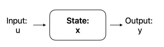
滤波步骤
| 变量 | input | predict | correct | output | 使用 |
|---|---|---|---|---|---|
| state | $\hat x_n$ | $x_n$ | [x,y,dx,dy] | ||
| measure | $u_n$ | $\hat y_n$ | $y_n$ | [x, y] |
| 参数 | 使用 | |
|---|---|---|
| transition matrix P | state -> predict state | \begin{bmatrix}1&0&1&0\\0&1&0&1\\0&0&1&0\\0&0&0&1\end{bmatrix} |
| measure matrix $C$ | state -> measure | \begin{bmatrix}1&0&0&0\\0&1&0&0\end{bmatrix} |
| gain $g_n$ | measure error -> state error | 根据仿真模型和运动模型更新 |
- predict:
- $\hat x_n=P(x_{n-1})$ 是state 在当前时间的predict
- correct:
- $x_{n}-\hat x_{n}=g_n\cdot(u_n-\hat y_{n})=g_n\cdot(u_n-C\hat x_n)$
- state的error和measure的error(measure-predict) 是线性关系
- 如果measure从predict偏移越少, state越保持predict的结果
- 写成SSM的形式: $x_n=\hat x_{n}+g_n\cdot(u_n-C\hat x_n)=(I-g_n\cdot C)\hat x_n +g_n\cdot u_n=(I-g_n\cdot C)P x_{n-1} +g_n\cdot u_n$
- state的error和measure的error(measure-predict) 是线性关系
- $x_{n}-\hat x_{n}=g_n\cdot(u_n-\hat y_{n})=g_n\cdot(u_n-C\hat x_n)$
通过运动模型更新gain $g_n$
| 变量 | 仿真 | predict | correct |
|---|---|---|---|
| state | $x_n^r$ | $\hat x_n^r$ | $\tilde x_n$ |
| error | $\hat \epsilon_n=x_n^r-\hat x_n^r$ | $\epsilon_n=x_n^r-\tilde x_n$ |
- 仿真模型:
- $x_n^r$ 是仿真的state
- $x_{n}^r=P(x_{n-1}^r)+ProcessNoise$(状态转移噪声)
- $u_n^r=C(x_n^r)+MeasureNoise$ 测量值仿真结果
- 假设ProcessNoise和MeasureNoise都是高斯分布的Random Variable
- 计算模型:
- predict:
- $\hat x_n^r=P(\tilde x_{n-1})$ 是predict值
- PredictError:
- $\hat \epsilon_n=x_n^r-\hat x_n^r=P(x_{n-1}^r)+ProcessNoise-P(\tilde x_{n-1})=P\epsilon_{n-1}+ProcessNoise$ ①
- correct:
- $\tilde x_{n}=\hat x_{n}^r+g_n\cdot(u_n^r-C\hat x_n^r)=\hat x_{n}^r+g_n\cdot(C\cdot \hat\epsilon_n+MeasureNoise)$ 是correct之后的state
- CorrectError:
- $\epsilon_n= x_n^r-\tilde x_n =\hat \epsilon_{n}-g_n\cdot( C\cdot \hat \epsilon_{n}+MeasureNoise)$ ②
- Gain: argmin(CorrectError)
- \[\begin{align}g_n=\text{argmin} ||x_{n}^r-\tilde x_{n}||&=\text{argmin} ||\hat \epsilon_n-g_n\cdot(C\cdot\hat \epsilon_n + MeasureNoise)||\\&=(\hat \epsilon_n)(C\hat \epsilon_n+MeasureNoise)^T((C\hat \epsilon_n+MeasureNoise)(C\hat \epsilon_n+MeasureNoise)^T)^{-1} & (\text{因为 }\text{argmin}||xA-b||=(bA^T)(AA^T)^{-1})\\&=(\hat \epsilon_n^{cov}C^T)(C\hat \epsilon_n^{cov} C^T+MeasureNoise^{cov})^{-1}&(\text{展开, }mean(MeasureNoise)=0)\end{align}\]
- predict:
- 特点:
- gain $g_n$ 和实际采集的数据$u_n$ 无关, 是由仿真过程和计算过程确定的
- ① , ② 为$\hat \epsilon_n$ 的更新过程
- 在gain的计算中, 每次更新$\hat \epsilon_n^{cov}, \epsilon_n^{cov}$ 就可以了
- gain 在一段时间后会收敛到一个固定的值
推导(Least Square)
定义 L2 norm: \(||A|| = ∑_{ij} A_{ij}^2 = trace(A^TA)\)
-
Normal Least Square: \(\min_x ||Ax-b|| = \min_x (Ax-b)^T(Ax-b)= \min_x (x^T(A^TA)x - 2x^T(A^Tb))\)
- 其中:
- $\partial_x x^T(G)x = 2Gx \ (\partial_{x_k} \sum G_{ij} x_i\cdot x_j = \sum G_{ik} x_i+\sum G_{kj} x_j\text{ related part are one for k-th row and one for k-th col)}$
- $\partial_x x^T(A^T b) = A^T b$
- 得到: $(A^TA)^{-1}(A^Tb)$
变形:
\[\text{argmin}_x ||xA-b||=\text{argmin}_{x^T} ||A^Tx^T-b^T||=((AA^T)^{-1}(Ab^T))^T=(bA^T)((AA^T)^{-1})^T=(bA^T)(AA^T)^{-1}\]